
Aim
To determine the overall and individual heat transfer coefficient under thermal steady state conditions.
Apparatus
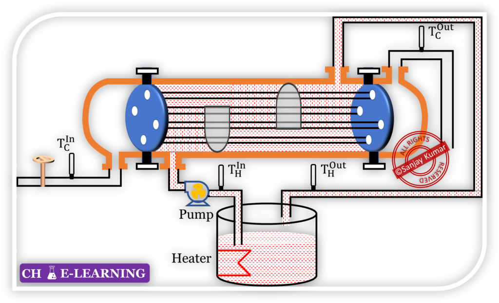
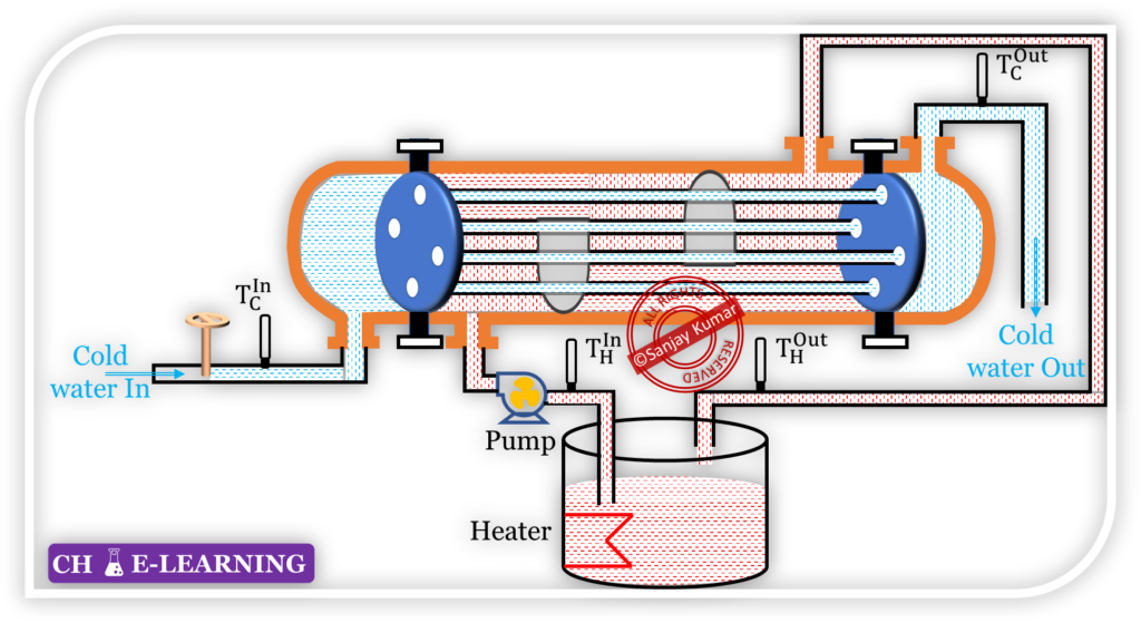
The experimental setup consists of a shell and tube heat exchanger, with multiple tubes enclosed within a cylindrical shell. The key components include:
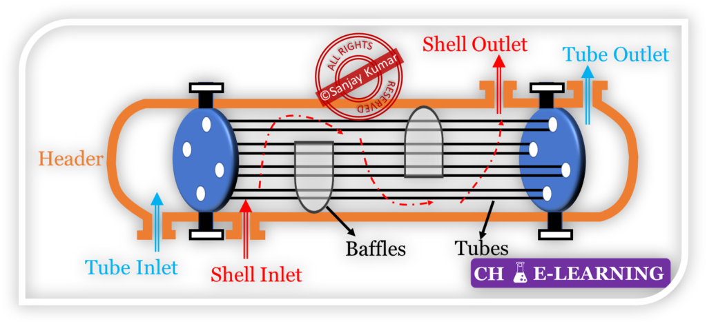
- Tube Bundle: A set of tubes through which the cold fluid flows.
- Shell: An outer cylindrical casing that allows hot fluid to flow around the tubes.
- Baffles: Internal structures placed within the shell to enhance heat transfer by directing the shell-side fluid flow and providing mechanical support to the tubes.
- Baffles increase the velocity and turbulence of the shell-side fluid, thereby improving the heat transfer.
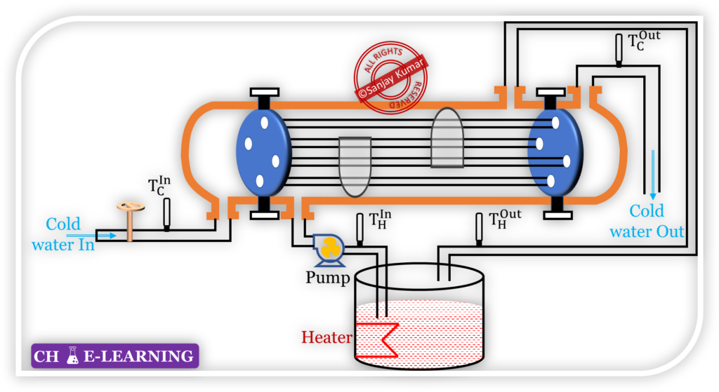
- Flow Control System: A cold-water inlet valve allows flow rate regulation.
- Thermometers: Measures the inlet and outlet temperatures of both hot and cold fluids.
- Pump: Facilitates hot water circulation through the shell.
- Hot Water Tank with Heater: Supplies hot water to the shell side of the exchanger.
- The hot water circulates through the shell and returns to the same tank.
- Schematic Diagram: A basic schematic for a single-pass shell-and-tube heat exchanger is shown in the Figure below.
Specifications:
The specifications for the 1-1 Heat exchanger are as follows:
- A 1-1 Heat exchanger refers to a 1-shell, 1-tube pass configuration.
- 1-Shell means a single shell enclosing the tube bundle.
- 1-tube pass means the fluid inside the tubes flows in a single pass from one end to the other end without reversing direction.
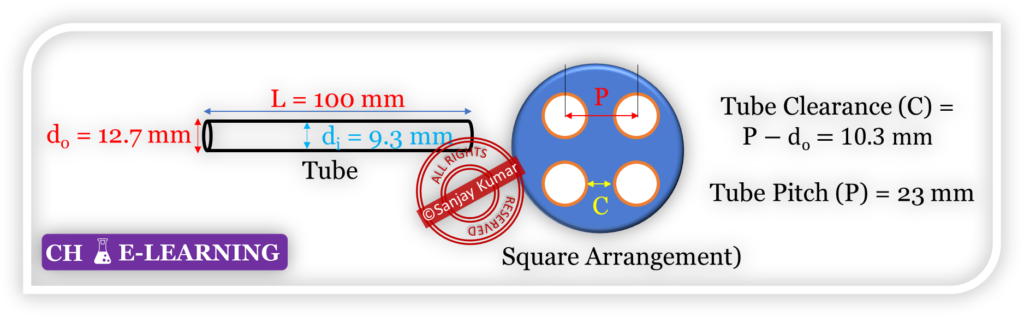
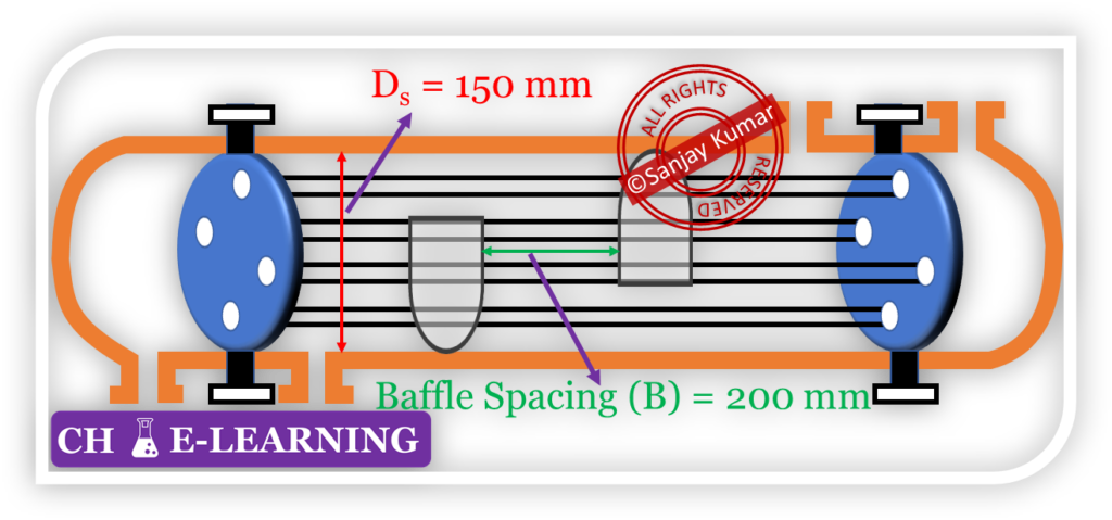
Geometric Specifications:
- No. of tube (N) = 37, Shell inside diameter (Ds) = 150 mm, baffle spacing (B) = 200 mm, length of each tube (L) = 600 mm, inner diameter of tube (di) = 9.3 mm, outer diameter of tube (do) = 12.7 mm, tube pitch (square arrangement) P = 23 mm, tube clearance C = (P – do) = 10.3 mm.
Malarial Properties:
- The shell material is stainless steel, and its thermal conductivity is k = 54 W/m.K
- The tube side material is copper, and its thermal conductivity is k = 386 W/m.K
Experimental Procedure
Steps are given below
Step 1: Hot Water Preparation)
- Fill the hot water tank with water up to approximately ¾ of its capacity.
- Turn on the heater and set the water temperature to 70 °C.
Step 2: Hot Water Circulation
- Once the set temperature (70 °C) is reached, start the pump to circulate hot water through the shell side.
- Wait until a steady-state condition is achieved, i.e., \mathrm{T_H^{In}=T_H^{Out}}
Step 3: Cold Water Circulation
- Open the cold-water inlet valve and adjust the flow rate. Cold water flows through the tube side.
- Monitor the outlet temperature of the cold water until a steady-state condition is achieved, i.e.,
\mathrm{T_C^{Out}=Constant}
- The flow rate of cold water can be estimated by collecting water for a given time.
Step 4: Data Collection
- Record the inlet and outlet temperatures for both hot and cold water.
Step 5: Repeat the Experiment
- Conduct the experiment for different cold water flow rates and note the readings.
Experimental Data
Record and tabulate hot and cold water temperature readings at varying cold water flow rates.
| Hot Water Reading (Shell-side) | |||
| Sr. No. | \mathrm{T_H^{In}(℃)} | \mathrm{T_H^{Out}(℃)} | \mathrm{T_H^{mean}(℃)=\frac{(T_H^{Out}+T_H^{In})}2} |
| 1 | 64 | 60 | 62 |
| 2 | 59 | 55 | 57 |
| 3 | 56 | 52 | 54 |
| Cold Water Reading (Tube-side) | ||||||
| Sr. No. | \mathrm{T_C^{In}(℃)} | \mathrm{T_C^{Out}(℃)} | \mathrm{T_C^{mean}(℃)} | Water collected (kg) | Time (s) | Mass flow rate \mathrm{{\dot m}_{bundle}\left(\frac{kg}s\right)} |
| 1 | 26 | 48 | 37 | 2.5 | 60 | 0.0417 |
| 2 | 26 | 42 | 34 | 3.4 | 60 | 0.057 |
| 3 | 26 | 39 | 32 | 4.1 | 60 | 0.0683 |
Experimental Overall H.T. Coefficient Calculations
Estimate the overall H.T. coefficient (Uoverall) based on the outside area of the tube using the Log Mean Temperature Difference (LMTD) method.
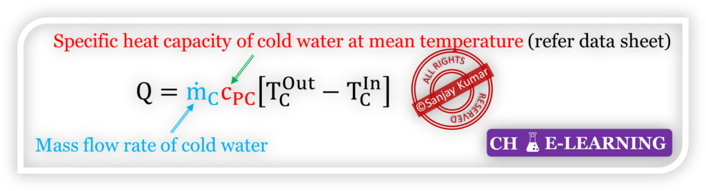
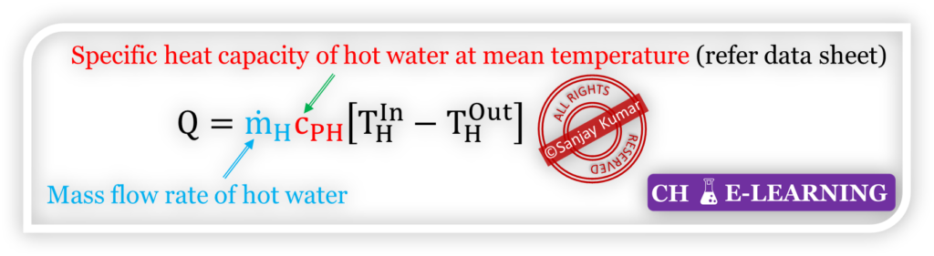
Step 1: Heat Load Calculation for Tube-side Flow
- Estimate the heat load for tube side flow using the equation given below.
| Heat Load Calculations for Different Flow Rates (Tube-side) | ||||||
| Sr. No. | \mathrm{T_C^{In}(℃)} | \mathrm{T_C^{Out}(℃)} | \mathrm{T_C^{mean}(℃)} | \mathrm{c_{PC}\left(\frac{kJ}{kg.℃}\right)} | \mathrm{{\dot m}_{bundle}\left(\frac{kg}s\right)} | Q (W) |
| 1 | 26 | 48 | 37 | 4.178 | 0.0417 | 3833 |
| 2 | 26 | 42 | 34 | 4.170 | 0.057 | 3803 |
| 3 | 26 | 39 | 32 | 4.1783 | 0.0683 | 3710 |
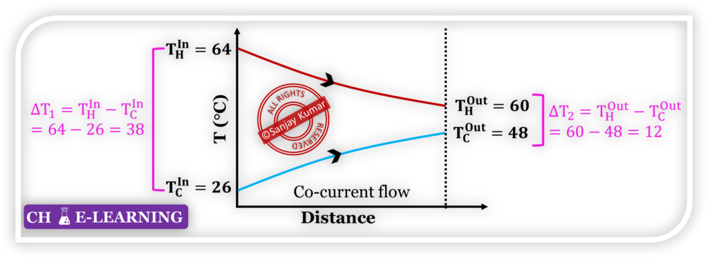
Step 2: LMTD Calculation for Co-current Flow
- The logarithmic mean temperature difference is calculated as:
\mathrm{ \triangle T_{LMTD}=\frac{\triangle T_1-\triangle T_2}{\ln\left({\displaystyle\frac{\triangle T_1}{\triangle T_2}}\right)} }
| LMTD Calculation | |||||||
| Sr. No. | \mathrm{T_C^{In}(℃) } | \mathrm{T_C^{Out}(℃) } | \mathrm{T_H^{In}(℃) } | \mathrm{T_H^{Out}(℃) } | ΔT1 | ΔT2 | LMTD (°C) |
| 1 | 26 | 48 | 64 | 60 | 38 | 12 | 22.56 |
| 2 | 26 | 42 | 59 | 55 | 33 | 13 | 21.47 |
| 3 | 26 | 39 | 56 | 52 | 30 | 13 | 20.33 |
Step 3: Estimate H.T. of Tubes
- The area of one tube can be written as
\mathrm{A_{tube}=\pi d_0L}
- For N number of tubes, the total H.T. area is:
\mathrm{A_{bundle}=N\pi d_0L}
- From specifications data: N = 37, d0 = 12.7 mm and L = 600 mm
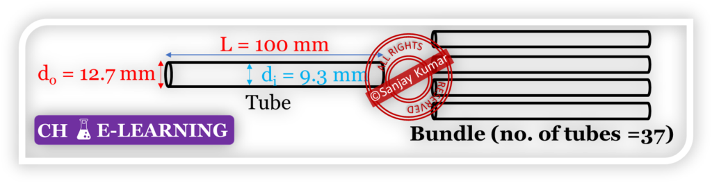
\mathrm {A_{tube}=37\times3.14\times12.7\times10^{-3}\times600\times10^{-3}=0.885\;m^2 }
Step 4: Estimate Overall H.T. Coefficient (Uoverall)
- Estimate the overall heat transfer coefficient using Q = UA(LMTD) equation.
\mathrm{ U_{overall}=\frac Q{A_{bundle}\times LMTD} }
| Q (W) | \mathrm{A_{bundle}\left(m^2\right)} | LMTD | \mathrm{U_{experimental}\left(\frac W{m^3.℃}\right)} |
| 3833 | 0.855 | 22.56 | 198.72 |
| 3803 | 0.855 | 21.47 | 207.17 |
| 3710 | 0.855 | 20.33 | 213.44 |
Theoretical Overall H.T. Coefficient Calculations
Tube-Side Film Coefficient:
Step 1: Properties of Cold Water at Mean Temperature
- Write the properties of cold water at a mean temperature from the datasheet.
| Cold Water Properties | ||||||
| Sr. No. | \mathrm{T_C^{mean}(℃) } | \mathrm{\rho\left(\frac{kg}{m^3}\right)} | \mathrm{\mu\left(\frac{kg}{m.s}\right)} | \mathrm{c_{PC}\left(\frac{kJ}{kg.℃}\right)} | \mathrm{k\left(\frac W{m.℃}\right)} | \mathrm{N_{Pr}=\frac{c_P\mu}\rho } |
| 1 | 37 | 993.3 | 0.0006 | 4.178 | 0.6232 | 4.608 |
| 2 | 34 | 994.3 | 0.0007 | 4.170 | 0.619 | 4.926 |
| 3 | 32 | 995.02 | 0.0007 | 4.1783 | 0.6162 | 5.1614 |
Step 2: Reynold’s Number Calculation
- Estimate the Reynolds number to determine the type of flow inside the tube-side using the equation:
\mathrm{N_{Re}=\frac{v\rho d_i}\mu}
- Since density, diameter (di = 9.3 mm), and viscosity are known, the velocity needs to be calculated.
- The velocity of fluid inside the tube-side across each tube is given by
\mathrm{{\dot m}_{tube}=\rho A_{tube}v}
- Since the total mass flow rate across the bundle is known, the mass flow rate across each tube can be estimated by dividing the total mass flow rate by the number of tubes (N = 37).
\mathrm{{\dot m}_{tube}=\frac{{\dot m}_{bundle}}{No.\;of\;Tubes\;(N)}}
- Inside cross-sectional area of a single tube is:
\mathrm{A_{tube}=\frac{\pi\left(d_i\right)^2}4=\pi\frac{\left(9.3\times10^{-3}\right)^2}4=6.79\times10^{-5}\;m^2}
| Sr. No. | \mathrm{{\dot m}_{bundle}\left(\frac{kg}s\right) } | \mathrm{{\dot m}_{tube}\left(\frac{kg}s\right) } | \mathrm{\rho\left(\frac{kg}{m^3}\right)} | \mathrm{A_{tube}\left(m^2\right)} | \mathrm{v\left(\frac ms\right) } | \mathrm{N_{Re}=\frac{v\rho d_i}\mu} |
| 1 | 0.0417 | 1.13×10⁻³ | 993.3 | 6.79 ×10⁻⁵ | 0.0167 | 224.55 |
| 2 | 0.057 | 1.54×10⁻³ | 994.3 | 6.79 ×10⁻⁵ | 0.0228 | 301.3 |
| 3 | 0.0683 | 1.85×10⁻³ | 995.02 | 6.79 ×10⁻⁵ | 0.0273 | 361.03 |
Step 3: Check Flow Nature
- For laminar flow (NRe < 2100), use the Graetz empirical equation:
\mathrm{N_{Nu}=1.86\left[N_{Gz}\right]^{1/3} }
\mathrm{Where,\;N_{Nu}=\frac{h_id_i}k;\;\;N_{Gz}=\frac{N_{Re}\times N_{Pr}\times d_i}L }
- For transition flow (2100 < Re < 4000), use a graphical method.
- For turbulent flow (NRe > 4000), use the Dittus-Boelter empirical equation:
\mathrm{N_{Nu}=0.023\left[N_{Re}\right]^{0.8}\left[N_{Pr}\right]^{0.4}}
Step 4: Estimate H.T. Coefficient (hi) Inside the Tube
- Use laminar flow empirical equation
| Sr. No. | NRe | NPr | di (mm) | L (mm) | NGz | NNu | \mathrm{k\left(\frac W{m.℃}\right)} | \mathrm{h_i\left(\frac W{m^2.℃}\right)} |
| 1 | 224.55 | 4.608 | 9.3 | 600 | 16.034 | 4.69 | 0.6232 | 314.28 |
| 2 | 301.3 | 4.926 | 9.3 | 600 | 23.08 | 5.17 | 0.619 | 344.37 |
| 3 | 361.03 | 5.1614 | 9.3 | 600 | 28.99 | 5.52 | 0.6162 | 370.96 |
Step 5: Estimate Adjusted Inside H.T. Coefficient (hio)
- It can be estimated using

- This correction is used when H.T. is analyzed in terms of the outside tube area instead of the inside. It is relevant when calculating the overall heat transfer coefficient, which is usually based on the outside area of the tube.
| Sr. No. | di (mm) | do (mm) | \mathrm{h_i\left(\frac W{m^2.℃}\right)} | \mathrm{h_{io}\left(\frac W{m^2.℃}\right)} |
| 1 | 9.3 | 12.7 | 314.28 | 230.14 |
| 2 | 9.3 | 12.7 | 344.37 | 252.18 |
| 3 | 9.3 | 12.7 | 370.96 | 271.65 |
Shell-Side Film Coefficients:
The heat transfer coefficients outside the tube bundle are referred to as shell-side coefficients.
Step 1: Properties of Hot Water at Mean Temperature
- Write the properties of hot water at mean temperature from the data sheet.
| Hot Water Properties | ||||||
| Sr. No. | \mathrm{T_H^{mean}(℃) } | \mathrm{\rho\left(\frac{kg}{m^3}\right)} | \mathrm{\mu\left(\frac{kg}{m.s}\right)} | \mathrm{c_{PC}\left(\frac{kJ}{kg.℃}\right)} | \mathrm{k\left(\frac W{m.℃}\right)} | \mathrm{N_{Pr}=\frac{c_P\mu}\rho } |
| 1 | 62 | 982.16 | 0.00044 | 4.18 | 0.653 | 2.855 |
| 2 | 57 | 984.71 | 0.00048 | 4.183 | 0.647 | 3.111 |
| 3 | 54 | 986.17 | 0.00006 | 4.182 | 0.6445 | 3.2814 |
Step 2: Estimate Shell-side Flow Rate
- Heat lost by shell side fluid will be equal to heat gained by tube side fluid.
\mathrm{Q_{Tube\;side}=Q_{Shell\;side}}
| Shell-side Flow Rate | ||||||
| Sr. No. | \mathrm{T_H^{In}(℃)} | \mathrm{T_H^{Out}(℃)} | \mathrm{T_H^{mean}(℃)} | \mathrm{c_{PC}\left(\frac{kJ}{kg.℃}\right)} | Q (W) | \mathrm{{\dot m}_{shell}\left(\frac{kg}s\right)} |
| 1 | 64 | 60 | 62 | 4.18 | 3833 | 0.229 |
| 2 | 59 | 55 | 57 | 4.183 | 3803 | 0.227 |
| 3 | 56 | 52 | 54 | 4.182 | 3710 | 0.222 |
NOTE: Since we are not changing the flow rate of shell-side water, the mass flow rate should remain practically constant. After calculation, the values are also nearly equal. The flow rate of hot water can also be estimated experimentally by collecting water for a given time.
Step 3: Find Reynold’s Number
- Estimate the Reynolds number to determine the type of flow inside the shell-side using the following equation:
\mathrm{N_{Re}=\frac{v\rho D_e}\mu=\frac{G_eD_e}\mu }
\mathrm{G_e\Rightarrow v\rho\Rightarrow\frac ms\frac{kg}{m^3}\Rightarrow\frac{kg}{m^2.s}\Rightarrow\frac{\dot m}{Area}}
- Here, inside the shell side, the fluid flow pattern is complex, so the simple Reynold equation can not be used. It is used in terms of effective mass velocity (Ge) and equivalent diameter (De).
- The effective mass velocity combines the mass velocities through the baffle window (Gb) and crossflow section (Gc)
\mathrm{G_e=\sqrt{G_b\times G_c}}
- Gb & Gc are the mass velocity through the baffle window & crossflow section respectively, calculated as
\mathrm{G_b=\frac{{\dot m}_{shell}}{S_b};\;\;G_c=\frac{{\dot m}_{shell}}{S_c}}
Where Sb is the flow area through the baffle window and Sc is the crossflow area between baffles.
\mathrm{S_b=f_b\left[Shell\;area-bundle\;area\right]=f_b\left[\frac{\pi D_i^2}4-N\frac{\pi d_o^2}4\right] }
Where fb = fraction of the shell’s cross-sectional area occupied by the baffle window (typically around 0.1955), Di = Shell inside diameter (150 mm), and do = tube outside diameter (12.7 mm).
\mathrm{S_b=0.1955\left[\frac{3.14\times\left(150\times10^{-3}\right)^2}4-37\frac{3.14\times\left(12.7\times10^{-3}\right)^2}4\right]=0.00254\;m^2 }
- The crossflow area between baffles can be estimated as
\mathrm{S_c=P\times D_i\left(1-\frac{d_o}P\right)}
Where P = tube pitch (23 mm), Di = Shell inside diameter (150 mm), and do = tube outside diameter (12.7 mm).
\mathrm{S_c=23\times10^{-3}\times150\times10^{-3}\left(1-\frac{12.7\times10^{-3}}{23\times10^{-3}}\right)=0.01343\;m^2 }
- Estimate the equivalent diameter of the shell for a square pitch can be estimated as
\mathrm{D_e=4\times\frac{Flow\;Area}{Wetted\;Perimeter}=4\times\frac{\left[P^2-{\displaystyle\frac{\pi d_0^2}4}\right]}{\pi d_0}}
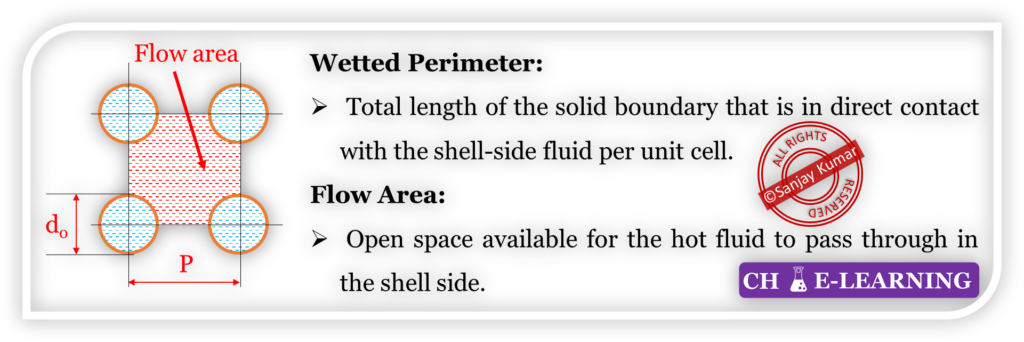
- From specifications data: P = 23 mm, do = 12.7 mm
\mathrm{ D_e=4\times\frac{\left[\left(23\times10^{-3}\right)^2-{\displaystyle\frac{3.14\times\left(12.7\times10^{-3}\right)^2}4}\right]}{3.14\times12.7\times10^{-3}}=0.04036\;m }
| Sr. No. | \mathrm{{\dot m}_{shell}\left(\frac{kg}s\right)} | Sb (m2) | Sc (m2) | \mathrm{G_b\left(\frac{kg}{m^2.s}\right) } | \mathrm{G_e\left(\frac{kg}{m^2.s}\right)} | De (m) | \mathrm{\mu\left(\frac{kg}{m.s}\right)} | \mathrm{N_{Re}=\frac{G_eD_e}\mu} |
| 1 | 0.229 | 0.00254 | 0.01343 | 90.157 | 39.209 | 0.04036 | 0.00044 | 3596.53 |
| 2 | 0.227 | 0.00254 | 0.01343 | 89.370 | 38.866 | 0.04036 | 0.00048 | 3267.98 |
| 3 | 0.222 | 0.00254 | 0.01343 | 87.402 | 38.010 | 0.04036 | 0.00006 | 25568.06 |
Step 4: Estimate Shell-side H.T. Coefficient (ho)
- Use Donohue’s empirical equation
\mathrm{N_{Nu}=0.2\left[N_{Re}\right]^{0.6}\left[N_{Pr}\right]^{0.3}}
\mathrm{Where,\;\;N_{Nu}=\frac{h_oD_e}k}
| Sr. No. | NRe | NPr | NNu | De (m) | \mathrm{k\left(\frac W{m.℃}\right)} | \mathrm{h_o\left(\frac W{m^2.℃}\right)} |
| 1 | 3596.53 | 2.855 | 37.260 | 0.04036 | 0.653 | 602.843 |
| 2 | 3267.98 | 3.111 | 36.097 | 0.04036 | 0.647 | 578.656 |
| 3 | 25568.06 | 3.2814 | 126.028 | 0.04036 | 0.6445 | 2012.511 |
Uoverall Theoretical Calculations:
Step 1: Find the Overall Theoretical H.T. Coefficient
\mathrm{\frac1{U_o}=\frac1{h_{io}}+\frac1{h_o}+R_w+R_d }
- Dirt resistance (Rd) can be neglected.
- Metal wall resistance (Rw) represents the resistance to heat conduction through the tube wall. It can be estimated as
\mathrm{R_w=\frac{d_o\ln\left({\displaystyle\frac{d_o}{d_i}}\right)}{2k_w}=\frac{12.7\times10^{-3}\times\ln\left({\displaystyle\frac{12.7}{9.3}}\right)}{2\times386}=5.13\times10^{-6}\frac{m^2.K}W }
Where di = inner diameter of tube (9.3 mm), do = outer diameter of tube (12.7 mm), and kw = thermal conductivity of tube (386 W/m.K).
| Sr. No. | \mathrm{h_{io}\left(\frac W{m^2.℃}\right)} | \mathrm{h_o\left(\frac W{m^2.℃}\right)} | \mathrm{R_w\left(\frac{m^2.K}W\right)} | \mathrm{U_{theoretical}\left(\frac W{m^2.℃}\right)} |
| 1 | 230.14 | 602.843 | 5.13×10⁻⁶ | 166.41 |
| 2 | 252.18 | 578.656 | 5.13×10⁻⁶ | 175.48 |
| 3 | 271.65 | 2012.511 | 5.13×10⁻⁶ | 239.05 |
Comparison of Experimental and Theoretical U:
The U represents the combined effect of conduction and convection heat transfer across a heat exchanger.
- While comparing experimental and theoretical values of U, we aim to understand how well our theoretical models predict real-world performance.
| Sr. No. | \mathrm{U_{experimental}\left(\frac W{m^2.℃}\right)} | \mathrm{U_{theoretical}\left(\frac W{m^2.℃}\right)} | Observation |
| 1 | 198.72 | 166.41 | Uexp > Utheo |
| 2 | 207.17 | 175.48 | Uexp > Utheo |
| 3 | 213.44 | 239.05 | Uexp < Utheo |